
Flooding gets into a building's wiring, stock and flooring; heat strains roofs and cooling systems; and strong wind loosens cladding and roofing. None of that physical damage arrives with a price tag attached and a risk officer reading a flood risk map or a heat exposure score does not get one either. This guide sets out the financial metrics that turn that exposure into a number a finance team will act on, then walks through one worked example showing exactly how.
How is physical climate risk quantified in financial terms?
Physical climate risk is quantified in financial terms using three standard catastrophe-modelling metrics: average annual loss (AAL), probable maximum loss (PML) and the percentage of total insured value (TIV) sitting in high-risk zones.
Physical climate risk itself is the potential for financial loss, operational disruption or asset damage that climate hazards such as flooding, extreme heat, high wind, water stress and wildfire cause to a business, whether through a sudden event or through gradual change over years.
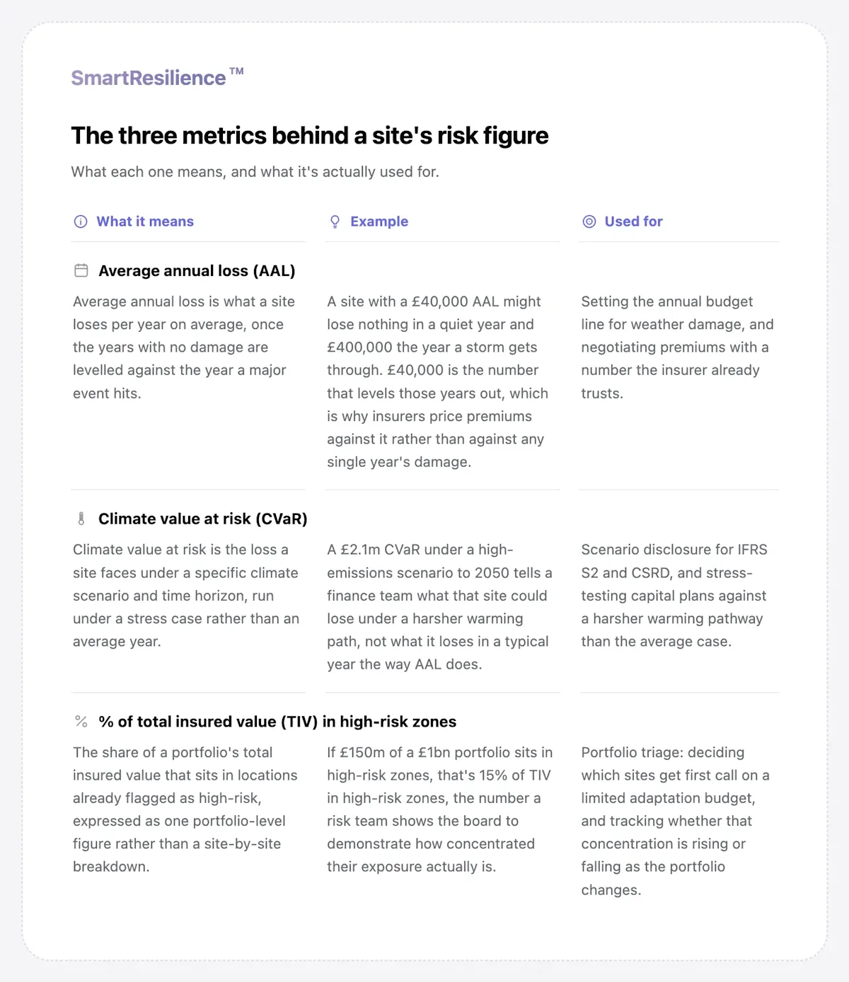
None of these are proprietary constructs. The Bank of England used AAL and PML as core outputs in its 2021 Biennial Exploratory Scenario, the stress test it ran on the UK's largest banks and insurers, because underwriters and investors already plan capital around them. A generic risk score of 62 out of 100 tells a finance director that exposure exists, not what it costs. AAL and PML tell that same finance director the cost, this year and in a bad year, which is the number a finance director can actually work with.
What data does a physical climate risk assessment need at site level?
A physical climate risk assessment needs three inputs to produce a financial figure: site-level asset data, hazard exposure data and a damage function connecting hazard severity to loss. A physical climate risk assessment is the process of working out which climate hazards each site faces, how much damage each hazard would cause and what that damage would cost, site by site and across the portfolio.
In practice, that means:
Site-level asset data: each site needs its own replacement cost, contents value and construction or elevation detail recorded individually, not folded into a regional or portfolio-wide average.
Hazard exposure data: modelled flood, heat, wind or water stress exposure gets mapped to those same site coordinates, drawn from a named dataset such as JBA's UK flood data or a CMIP6 (Coupled Model Intercomparison Project Phase 6) model ensemble, rather than a generic regional estimate.
A damage function: a documented curve links a given hazard severity, for example 40cm of flood depth, to an expected percentage of asset damage, calibrated against historical claims where they exist.
A stated time horizon and emissions pathway: the calculation needs a stated future date and warming scenario (the global temperature rise it assumes, for example 1.5°C or 3°C above pre-industrial levels) to run against, since both change the result materially.
This is physical risk, the direct damage a hazard does to an asset. It sits apart from transition risk, the cost of a shift to a low-carbon economy, which draws on a different set of inputs entirely and stays out of scope here.
How does scenario analysis change AAL and PML over time?
Scenario analysis changes these numbers by running the same site's hazard exposure through more than one possible climate future, each defined by an emissions pathway and a time horizon, rather than relying on a single set of assumptions. AAL and PML shift across those futures because hazard frequency and severity themselves change with the pathway and time horizon chosen.
What shifts, and why:
Emissions pathway
This is a modelled trajectory of how much greenhouse gas the world emits going forward, from steep near-term cuts to continued high emissions. A higher-emissions pathway produces more frequent and severe hazard events by the same future date than a lower-emissions pathway.
Time horizon
This is the future date or period a calculation is run against. A team calculating against 2030 conditions understates exposure by 2050 or 2080, because hazard intensity keeps changing across that period.
Portfolio and asset changes
When a team acquires new sites, disposes of others or completes adaptation measures, the numbers move independently of the climate data itself.
The IPCC (Intergovernmental Panel on Climate Change)'s Sixth Assessment Report, Working Group I documents how several acute hazards are already shifting in frequency and intensity as the climate warms, exactly the movement a single fixed AAL calculation cannot capture. Running the same site through more than one pathway produces a range rather than one number, which is closer to how a finance team should treat any forward-looking figure. The fuller mechanics of running this properly across pathways and time horizons sit in SmartResilience's guide to scenario analysis for climate resilience.
What does the calculation look like for one site, step by step?
The calculation runs in four steps for one site: mapping the hazard, applying a damage function, calculating AAL and PML, then comparing adaptation options against the loss they avoid.
Take one composite site inside a wider multi-country portfolio: a distribution centre insured for £20m, sitting in a mapped UK flood zone. Run it through the four steps below and a finance team gets an AAL of roughly £150,000 a year and a 1-in-100-year PML of around £4.0m, the two figures a finance team can put directly into a budget and a capital plan.
Map the hazard exposure: UK flood data for this location puts the annual probability of a 40cm flood at around 1-in-30, and a 1-in-100-year event at closer to 95cm.
Apply a damage function: A documented damage curve for this asset class translates 40cm of flood depth into roughly 9% of insured value damaged, and 95cm into roughly 20%.
Convert to AAL and PML: Weighting each depth by its annual probability across the full range of modelled events, from shallower and more frequent flooding to events rarer and deeper than the 1-in-100, produces an AAL of around £150,000 a year, or 0.75% of the site's TIV. The 1-in-100-year scenario alone produces a PML of about £4.0m, around a fifth of the site's TIV.
Compare adaptation options by ROI (return on investment): A flood barrier and improved drainage costed at £150,000 cuts this site's AAL by roughly 65%, to around £52,500 a year, an avoided-loss payback of roughly 18 months, before counting any reduction in insurance excess that tends to follow.
Practical tip: ask for AAL and PML at individual site level across a representative sample of the portfolio, not a single blended average. A number that cannot be traced back to a specific site and a specific assumption is difficult to defend to finance, or to a divisional lead who doubts it.
How does this differ from a one-off consultancy report?
A one-off consultancy report differs from the calculation just walked through in what happens after delivery: the report is fixed at a single portfolio snapshot, while the same calculation can be rerun whenever hazard data, portfolios or climate science change.
What changes when a team reruns the calculation instead of receiving it once:
Update cadence: a consultancy engagement typically reruns every 12 to 24 months, while a team on a live platform recalculates the figure as new hazard data and portfolio changes arrive.
Audit trail: a static report usually arrives as a PDF with a methodology annex, while a live platform shows the data lineage behind every AAL and PML figure, so a finance team can check a number rather than take it on faith.
Cost of the next update: a fresh consultancy engagement tends to cost close to the first one, while a team can refresh a live platform's inputs without recommissioning the whole exercise.
How do these numbers support disclosure and adaptation decisions?
AAL, PML and % of TIV support three separate decisions: what a sustainability team discloses, what evidence a risk team takes into an insurance renewal and where a facilities or risk team spends on physical adaptation measures such as flood barriers or drainage upgrades.
Where each figure gets used:
Disclosure: IFRS S2 (the International Sustainability Standards Board's climate-related disclosure standard) and the IFRS S2 aligned UK SRS (UK Sustainability Reporting Standards) S2 both ask organisations to report the amount and percentage of assets or business activities vulnerable to physical risks. A sustainability team can answer that with % of TIV in high-risk zones by hazard, backed by AAL, PML and scenario-based exposure to 2080-2100.
Insurance renewal: a site-level AAL or PML figure gives a risk team specific evidence to put in front of an insurer, which tends to carry more weight at renewal than a general description of the risk.
Adaptation ROI: the same AAL and PML figures let a team compare adaptation measures on a like-for-like basis, weighing an avoided annual loss against the capital a measure costs, rather than ranking options by instinct.
How SmartResilience helps you quantify physical climate risk
SmartResilience Climate Assessments calculate the figures in this guide for every site in your portfolio, straight from your site data. Each number traces back to named sources, including IPCC AR6 emissions pathways and JBA UK flood data, and your team can export the full calculation for audit.
For your organisation, that means:
Site-level financial output, not a risk score: every site in the portfolio carries an AAL, a PML and a %TIV reading by hazard, generated using the same method walked through in the worked example above.
Scenario-based exposure to 2080-2100: modelled against whichever emissions pathway the organisation already uses for other reporting, so the figures stay consistent across finance, risk and sustainability teams.
Adaptation options ranked by ROI: indicative adaptation capex for the highest-risk sites, ranked so facilities and finance teams can prioritise together rather than negotiate site by site.
Continuously updated, not delivered once: new hazard data and portfolio changes feed the same figures automatically, so a number used in this year's board pack is not two years old by the time someone checks it.
Sainsbury's shows what changes when site-level risk information reaches the people running each site. Early warning runs across more than 1,000 of its sites, and ahead of Storm Franklin in February 2022 its teams in a town Storm Eva had flooded in 2015 had 12 hours' notice. They came through with no damage to property or stock and were operating again the next day, avoiding a loss estimated at £3m.
SmartResilience
See SmartResilience in action
Book a free demo tailored to your organisation and assets.
Book a free demoWhat next?
Analysts revise climate data, portfolios shift and facilities teams install or delay adaptation measures, so a physical risk figure calculated once already lags behind reality by the time it reaches a board pack. The decision now in front of most sustainability teams is not whether to quantify physical climate risk financially, but how often the resulting numbers need to move to stay credible with finance, and who outside sustainability sees them change.
Frequently Asked Questions (FAQs)
Does quantifying physical climate risk affect insurance premiums?
Insurers increasingly price site-specific evidence into renewal terms rather than accepting a general risk narrative. A renewal conversation backed by an AAL or PML figure, alongside evidence of adaptation measures already in place, tends to secure better terms than one built on a qualitative description alone.
How accurate are AAL and PML, given they are modelled rather than measured?
They are estimates built from historical hazard data and damage curves, not direct measurements, so accuracy depends on the quality of the underlying data and how transparently the assumptions are documented. A methodology with visible data lineage lets a team check and challenge each assumption, rather than accept a number on trust.
How often should physical climate risk be recalculated?
At minimum annually, and immediately after any site acquisition, disposal or major weather event, since portfolio changes and updated hazard data both shift the underlying figures. Treat monitoring as part of the exercise, not a separate project scheduled for next year.
Can this be done without commissioning a full consultancy engagement each time?
Site-level hazard data, a damage function and the underlying calculations are available through specialist platforms without recommissioning a full engagement for every update. A consultant remains useful for interpreting results or building an internal business case, but the calculation itself does not require one each time.
Does every site need the same level of financial modelling detail?
No. A portfolio triage using % of TIV by hazard usually narrows a large estate down to a smaller set of high-exposure sites that warrant full AAL and PML modelling, so effort concentrates where the financial exposure actually sits.